Reinforcement learning (RL), a pivotal subfield within artificial intelligence (AI), has achieved remarkable breakthroughs in autonomously solving complex tasks. It operates on the principle of training an intelligent "agent" to accomplish a goal through iterative trial and error. This agent, a sophisticated computer program, continuously observes its environment, makes strategic decisions on subsequent actions, and refines its decision-making framework, known as its "policy," based on received feedback. The feedback, typically a numerical "reward," guides the agent towards optimal behavior, whether it’s accumulating points in a video game, securing victory in a chess match, or enabling a robot to take a stable step without toppling over. This iterative process of observation, action, reward, and policy refinement allows the agent to progressively enhance its performance over countless interactions with its environment.
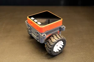
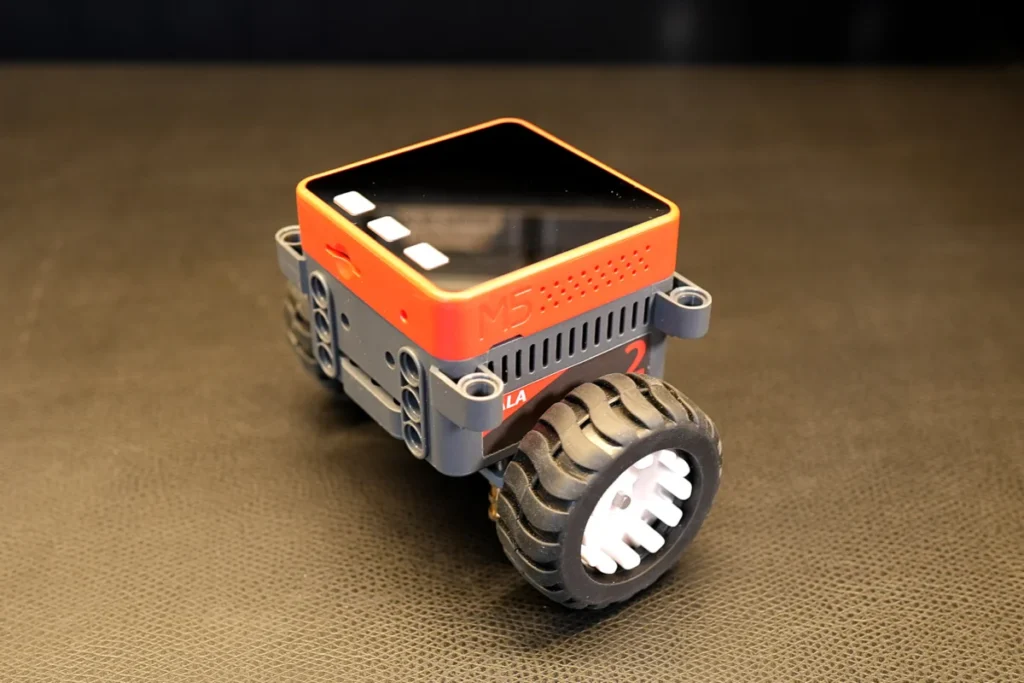
While traditional control schemes such such as proportional-integral-derivative (PID) loops, linear-quadratic regulators (LQR), and model predictive control (MPC) have long been the bedrock of engineering, RL is rapidly gaining prominence, particularly in the dynamic realm of robotics. Although setting up, training, and deploying an RL agent to a physical robot can present intricate challenges, the resulting controllers exhibit unparalleled robustness and adaptability to environmental variations. Unlike classical methods that demand precise mathematical modeling of every conceivable state or scenario, an RL agent can be trained to generalize across a vast spectrum of situations, empowering robots to navigate and respond effectively to similar, previously unencountered conditions. This guide will provide a conceptual overview of reinforcement learning before demonstrating how to train a self-balancing robot using the widely acclaimed Proximal Policy Optimization (PPO) algorithm. While the challenge of balancing a two-wheeled robot has been effectively addressed by classical control methodologies, this exercise serves as an accessible introduction to core RL principles, offering a hands-on experience in training an RL agent within a few hours, thereby preparing enthusiasts for more complex robotic endeavors, such as the bipedal Microduck developed by Pollen Robotics/Hugging Face. The majority of this tutorial can be completed using a standard computer for simulated training, with the option to deploy the learned policy to real hardware, specifically an M5Stack Bala2-Fire self-balancing robot kit, for tangible results.
A Historical Trajectory of Reinforcement Learning
The foundational concepts of reinforcement learning trace back to the 1950s, influenced by pioneering research in dynamic programming by Richard Bellman and early explorations into computational trial-and-error learning by Marvin Minsky. Arthur Samuel’s iconic checkers-playing program, also from this era, exemplified the early promise of machines learning from experience. Much of this nascent work drew inspiration from animal learning theories, notably Edward Thorndike’s law of effect, which posits that responses followed by satisfaction are more likely to recur, and B.F. Skinner’s operant conditioning, focusing on learning through rewards and punishments.
For several decades, RL research primarily centered on algorithms that could learn from direct experience rather than relying on a complete, explicit mathematical model of the environment. Bellman’s dynamic programming, while powerful, proved effective mainly when the world’s behavior was perfectly known and the number of possible states was computationally manageable—a rare luxury in real-world applications. Even games with well-defined rules, like chess or Go, possess an astronomically large number of possible positions, making exact calculation impractical. A significant breakthrough occurred in 1992 with IBM’s Gerald Tesauro, who combined temporal-difference learning with a neural network to create TD-Gammon. This program famously taught itself backgammon through self-play, achieving a near-world-champion level and demonstrating the potent synergy between learning from experience and neural network representation. The real world, however, presented even greater challenges than board games, with its immense variability, sensor noise, motor backlash, and unpredictable external disturbances, making precise modeling virtually impossible for tasks like robotic arm manipulation.

The advent of the deep learning revolution in the early 2010s marked a profound turning point for RL, ushering in the era of deep reinforcement learning. In this paradigm, neural networks are leveraged to estimate future rewards from given situations, represent the policy itself, or perform both functions simultaneously. This computational leap catalyzed a rapid succession of RL successes. Many scholars pinpoint 2013 as the crucible of this deep RL revolution, when DeepMind’s Deep Q-Network (DQN) learned to master dozens of Atari video games by directly analyzing raw pixel data, showcasing the power of end-to-end learning.
The impact of deep RL extended far beyond simple video games. In 2016, DeepMind’s AlphaGo stunned the AI community by defeating Lee Sedol, one of the world’s top Go players, in a historic five-game match, underscoring RL’s capacity for complex strategic reasoning. This was followed in 2019 by OpenAI Five, another RL program, which triumphed over the professional eSports team OG in the popular video game Dota 2, demonstrating mastery in a highly complex, real-time, multi-agent environment.
More recently, deep RL has permeated various domains beyond gaming. It has become instrumental in fine-tuning large language models (LLMs) like ChatGPT and Claude through techniques such as Reinforcement Learning from Human Feedback (RLHF), ensuring these models generate responses that are more helpful, honest, and harmless. In robotics, deep RL is driving unprecedented progress. In 2024, Boston Dynamics announced the integration of RL into the locomotion controller of its renowned quadruped robot, Spot, complementing the classical MPC it had employed for years. This move highlights RL’s contribution to enhanced robustness and agility. In the same year, Disney Research published findings on its BDX droids, which utilize RL to execute expressive, animator-designed movements, imbuing them with lifelike personalities and greater emotional range. The adoption of RL by such prominent organizations underscores its transformative role in advancing the field of robotics, demonstrating its practical efficacy in bridging the gap between simulated learning and real-world performance.
The Foundational Reinforcement Learning Loop
Reinforcement learning fundamentally operates through a relatively straightforward, yet powerful, learning loop. At its core, the "agent" embodies the decision-making logic. Auxiliary code components handle sensor data acquisition (e.g., from IMUs, motor encoders, or camera pixels) and preprocess this information into an "observation," which is then fed to the agent. Based on this observation, the agent’s "policy" dictates the "action" to be taken. This action serves as the control signal for the system, whether it involves adjusting game character inputs, recommending a movie, executing a stock trade, or, in the context of our balance bot, setting the speed and direction of its motors.
Crucially, the "agent" refers specifically to the algorithmic core comprising the decision-making policy, any value estimation components, and the learning algorithm itself responsible for updating these internal mechanisms. Conversely, the "environment" encompasses everything else: the supporting code that interfaces with sensors and calculates rewards, the physical actuators (motors), electronics, robot chassis, and the entire external world with which the robot interacts.

Upon executing an action, the environment responds dynamically. For the balance bot, motor activation leads to wheel rotation, causing the robot to tilt or move. The supporting code then captures new sensor readings, forming the subsequent observation for the agent. Concurrently, during the learning phase, a "reward" signal is generated, quantifying the environment’s reaction to the agent’s previous action. For the balance bot, this reward is a single numerical value derived from a combination of factors, including the robot’s pitch (deviation from vertical), the magnitude of the actions taken, its horizontal position, its translational speed, and its yaw rate (rotational speed).
The learning algorithm, in this example PPO, leverages these rewards to systematically update the agent’s internal parameters, with the ultimate goal of optimizing future actions to maximize the total cumulative rewards collected over time. Once the agent’s performance reaches a satisfactory level, it can be deployed to the actual robot or a high-fidelity simulation. Typically, only the "policy" portion of the agent (often termed the "actor" in deep RL) is deployed, as the "value estimator" (or "critic") is primarily a training aid. The deployment code also often omits the reward calculation, as the objective shifts from learning to executing optimal actions based solely on observations.
A critical aspect of this process is performing learning in a simulated environment, offering benefits such as safe resets upon failure, accelerated physics computations, and the ability to run multiple parallel environments to drastically speed up training. However, successful "sim-to-real" transfer—applying a policy learned in simulation to a real robot—demands meticulous attention. Observation values from the real robot must precisely align with those seen in simulation, necessitating identical filtering, normalization, and unit conversions. For instance, if simulated acceleration uses m/s² and real sensors provide g-force, a conversion is essential before feeding data to the agent. Similarly, policies usually output normalized actions (e.g., -1 to 1). This must be scaled consistently: a simulated "full power forward" (1.0) must correspond to the maximum PWM signal for the real motor driver. Clipping policy outputs within the expected range (-1 to 1) before scaling is also a good practice to prevent unintended behavior from extreme values. Consistency between simulation and reality is paramount for effective deployment.
Unpacking Proximal Policy Optimization (PPO)
The vast landscape of RL algorithms offers dozens of potent methods, and selecting the optimal one can be an art in itself. For this demonstration, Proximal Policy Optimization (PPO), introduced in a seminal 2017 paper by OpenAI researchers, is employed. PPO remains one of the most popular and effective RL algorithms for robotic control and LLM fine-tuning today. While its mathematical underpinnings are extensive, a conceptual understanding of its mechanics is crucial. Reference implementations, such as those found in Costa Huang’s cleanrl repository, provide valuable insights into its structure.
PPO is categorized as an "actor-critic" method, leveraging two distinct neural networks within the agent architecture:

-
The Critic Network: This neural network takes the environment’s "observation" (representing the "state"—either full or partial, like our robot’s sensors which cannot detect wheel slippage) as its input. The critic’s primary function is to answer the fundamental question: "How good is this state?" In complex, stochastic environments like a robot navigating the real world, precisely modeling environmental responses to actions is often intractable due to sensor noise, motor variations, and unmodeled physics. Instead of modeling the environment directly, the critic learns a simpler yet powerful approximation: an estimate of the total future reward expected from a particular state.
During interactions with the environment (or simulation), a log of actions, observations, and rewards—termed a "rollout"—is collected. This rollout data is then used to train the critic to predict the cumulative future rewards, known as the "return." In practice, future rewards are often "discounted" by a "gamma value," making immediate rewards slightly more valuable than distant ones, which encourages quicker goal achievement and prevents infinitely growing returns. The critic’s internal parameters are updated using the standard neural network training algorithm, "backpropagation," to improve its accuracy in predicting future returns. As rollouts accumulate, the critic refines its predictions, moving from random guesses to increasingly accurate estimations of total cumulative rewards for any given state, information critical for the actor.
-
The Actor Network: This neural network serves as the agent’s "policy." Like the critic, it receives an observation as input at each timestep. However, instead of estimating state value, the actor outputs the suggested action. For continuous control tasks, such as regulating motor speeds, the actor typically provides a "mean" value for each action, paired with a "standard deviation" to define a Gaussian (normal) "probability distribution." In some PPO implementations, the actor directly outputs both mean and standard deviation; in others, like CleanRL, the actor network computes the mean, while the standard deviation is a separate, learnable parameter for each action. During training, the agent samples a random action from this distribution.
This probabilistic approach offers a crucial advantage: it allows for explicit control over the "exploration-exploitation" tradeoff during training. Initially, the actor might output a broad standard deviation, signifying uncertainty and encouraging diverse "exploration" of actions ("I don’t know the best action, so try various ones"). As the agent accumulates experience and learns which actions yield higher future returns, the actor’s mean output shifts towards optimal actions, and its standard deviation shrinks, transitioning from broad exploration to focused "exploitation" of known-good options.
The actor, like the critic, is trained via backpropagation. Its objective is to maximize the returns generated by its chosen actions. Lacking a perfect model of the environment, the actor relies on the critic’s predictions to gauge the potential value of a given action. After an action is taken, the "advantage" is calculated—the difference between the actual outcome and the critic’s predicted outcome. If an action leads to a better-than-predicted result, the actor adjusts its policy to make that action more probable in similar future states; conversely, if the outcome is worse, the action becomes less likely.
Thus, the actor and critic collaborate: the critic approximates the total expected return from a state (assuming the actor’s policy is followed), while the actor uses this information to select actions that maximize that total return. Actor-critic methods are exceptionally powerful for learning complex behaviors in environments that defy complete mathematical modeling. However, their interdependency makes them highly sensitive to "hyperparameters"—the manual settings like learning rate and gamma, distinct from the automatically updated network parameters.

PPO’s key innovation lies in its mechanism for maintaining learning stability. After each rollout, PPO reuses the collected data for multiple rounds of updates. A challenge here is that this data was generated by an older version of the policy. If the policy changes too drastically between updates, the data becomes stale and no longer accurately reflects the agent’s behavior, potentially leading to catastrophic "bad updates." PPO mitigates this through "clipping," which limits the magnitude of policy updates. This acts as a "speed limit" on learning, ensuring the agent improves in measured, safe increments rather than unstable, risky leaps, thereby enhancing both stability and efficiency.
Setting Up the Environment for Balance Bot Training
To embark on the practical training of our balance bot, we will leverage Google Colab, a free cloud-based runtime environment for Python, eliminating the need for local software installations. The training will utilize MuJoCo, a robust physics simulator, to model the robot’s interactions. The specific Colab notebook, located at colab.research.google.com/github/shawnhymel/make-reinforcement-learning-for-robotics/blob/main/software/make_rl_train_balance_bot.ipynb, guides the process through a series of "cells" in a Jupyter Notebook format.
The initial cells are dedicated to installing and importing necessary libraries. These include custom libraries from the github.com/ShawnHymel/make-reinforcement-learning-for-robotics repository, which contains the environment definition (balance_bot_env.py) and the robot’s physical model (balance_bot.mjcf). Subsequently, a series of cells configure various training settings and hyperparameters. For instance, the system is configured to train the robot across eight separate, parallel environments, significantly accelerating the learning process. Each environment will run for 500,000 total timesteps, with each timestep involving an action, observation, and reward calculation, which then feeds into the actor and critic updates. PPO-specific hyperparameters define the actor and critic networks, each featuring two hidden layers with 32 nodes. Setting the timestep value to 0 allows the simulation to run as fast as the computational resources permit, often much quicker than real-time.
Helper functions are provided to create environments from the custom libraries, generate evaluation videos showcasing the policy’s performance, and load previously saved agents. Before commencing full training, two preliminary tests are conducted: one recording a video of the robot falling without any policy (demonstrating the baseline instability) and another showing the robot’s erratic movements under a random policy. These initial visualizations help confirm the environment setup is correct.
Crafting the Reward Function: The Art of Shaping Behavior

The reward function is the bedrock of reinforcement learning, directly shaping the agent’s behavior. In "Phase 1: Balance only," the initial training phase, the balance bot’s reward function is meticulously designed with specific coefficients:
envs = make_envs(
    NUM_ENVS,
    pitch_penalty_coef=0.5,
    action_penalty_coef=0.01,
    position_penalty_coef=0.001,
    speed_penalty_coef=20.0,
    yaw_penalty_coef=0.1,
)
Within the balance_bot_env.py file, the reward function is constructed as follows:
# Compute the penalties
pitch_penalty = self.pitch_penalty_coef * pitch**2
action_penalty = self.action_penalty_coef * np.sum(action**2)
position_penalty = self.position_penalty_coef * (x_pos**2 + y_pos**2)
speed_penalty = self.speed_penalty_coef * (x_vel**2 + y_vel**2)
yaw_penalty = self.yaw_penalty_coef * abs(yaw_rate)
# Reward function: subtract penalties from the alive bonus
reward = self.alive_bonus - pitch_penalty - action_penalty - position_penalty -
         speed_penalty - yaw_penalty
At each timestep, this function calculates a single numerical reward based on the current state. A positive value indicates a reward, while a negative value signifies a penalty. Let’s dissect each component:
alive_bonus(default 1.0): This constant positive reward is given at every timestep the robot remains upright. It fundamentally encourages the agent to prolong its active state, preventing it from immediately falling.pitch_penalty: This term penalizes the robot for tilting away from a perfectly upright position. The squared pitch value ensures that even small deviations incur a penalty, and larger deviations are penalized exponentially more, strongly incentivizing vertical balance.action_penalty: This penalty discourages the agent from taking overly aggressive or large actions. By penalizing the sum of squared motor actions, it promotes smoother, more energy-efficient movements, which are often desirable for stable control.position_penalty: This term penalizes the robot for moving away from its initial starting position. It encourages the robot to balance in place rather than drifting or rolling across the floor.speed_penalty: Similar to the position penalty, this term penalizes the robot for translational movement. A high coefficient here strongly incentivizes the robot to remain stationary.yaw_penalty: This penalty discourages the robot from rotating around its vertical axis. It ensures the robot maintains its heading while balancing.
Each reward and penalty is scaled by a coefficient, providing critical "hyperparameter knobs" to tune the robot’s behavior. Designing an effective reward function is often an art, requiring careful consideration to avoid "reward hacking"—scenarios where the agent discovers a way to maximize its reward without achieving the programmer’s intended outcome. For instance, if only an alive_bonus and pitch_penalty were present, the agent might learn to roll on its side to stay "upright" (from its internal perspective), thereby earning maximum reward without balancing. The inclusion of position_penalty and yaw_penalty helps mitigate such unintended behaviors.
Throughout the training phases, the "TensorBoard" visualization toolkit is indispensable. The most crucial graph to monitor is charts/episodic_return, which displays the total cumulative reward for each simulation episode (before the robot falls or time expires). This value should ideally converge towards a maximum (10,000 in this case), indicating the agent has discovered an optimal policy. Once Phase 1 shows the robot balancing effectively in the evaluation video, the process moves to Phase 2. It’s important to note Colab’s runtime limits (typically 12 hours) and potential disconnections, requiring session restarts and retraining.
Bridging the Sim-to-Real Gap with Domain Randomization and Curriculum Learning

After successfully training the robot to balance in simulation during Phase 1, a significant challenge remains: transferring this learned behavior to the real world. The "sim-to-real gap" arises from the inherent discrepancies between idealized simulations and physical reality, including unmodeled physics, sensor noise, variations in component tolerances, and environmental unpredictability.
One of the most powerful techniques in RL to address this gap is "Domain Randomization (DR)." Instead of attempting to perfectly model the real world in simulation—often an impossible feat—DR involves systematically varying numerous properties of the simulated environment and robot. The agent, therefore, learns to operate effectively across a wide range of conditions, becoming robust to these variations while still optimizing its reward function. As long as the real robot’s characteristics fall within the randomized ranges, the learned policy should generalize. A simple, easily visualized example of DR is adding random "nudges" to the simulated robot, mimicking external disturbances or minor collisions, forcing the agent to learn recovery strategies.
Rather than randomizing all properties simultaneously from the outset, which can overwhelm the agent, we employ "curriculum learning." This technique involves training the agent in progressively more challenging phases, gradually increasing task difficulty or introducing more DR elements. Without curriculum learning, an agent might struggle to learn complex tasks or converge on suboptimal "reward hacking" behaviors. Curriculum learning allows us to incrementally shape the agent’s behavior.
The process begins by using the agent trained in Phase 1 as the starting point for "Phase 2: Domain randomization for controls." Here, DR is introduced for internal robot control and electronic parameters:
- Sensor noise: Simulates the inherent inaccuracies of real-world sensors.
- Action delay: Models the latency between a command being issued and its physical execution by motors.
- Motor noise: Accounts for inconsistencies in motor performance.
- Motor torque variation: Simulates fluctuating battery charge levels affecting motor power.
Training for Phase 2 typically takes another 20-30 minutes. Post-training, monitoring the charts/episodic_return in TensorBoard is essential to ensure the agent maintains its high reward performance. The evaluation video should confirm the robot still balances stably despite the introduced variability. It’s a common practice to save the best-performing agent from each phase, ensuring continuity of progress even if the agent’s performance fluctuates towards the end of a training run.
Following successful completion of Phase 2, the process proceeds to "Phase 3: Domain randomization for the physical world." This phase introduces additional external DR properties:

- Random nudges: Further simulating external forces or collisions.
- Varying part masses: Accounting for slight manufacturing differences or measurement inaccuracies in robot components.
- Varying wheel-ground friction: Mimicking different surface types the robot might encounter (e.g., carpet, wood, tile).
Again, TensorBoard charts and evaluation videos are crucial for verifying the robot’s intended behavior—balancing upright without excessive movement or turning. Once satisfied with the performance, the final cells in the "Clean up and save model" section are executed, marking the completion of the balance bot agent’s training.
Deployment to Real Hardware
The culmination of the training process involves deploying the learned agent to the physical M5Stack Bala2-Fire robot. For deployment, only the "actor" neural network is required, as the "critic" was solely a training aid. The actor’s output, representing the mean of the action probability distribution, is used directly as the suggested action, with the standard deviation being discarded. The trained actor is exported as both an ONNX (Open Neural Network Exchange) file for cross-platform inference and a .h header file for C, facilitating integration into embedded systems. The actor.h file, containing the automatically generated neural network code, is then copied into the make-reinforcement-learning-for-robotics/software/balance_bot_arduino directory, overwriting any existing placeholder.
Using the Arduino IDE, with the M5Unified library and M5Stack board definitions installed, the balance_bot_arduino.ino sketch is opened. This sketch orchestrates the robot’s real-time operation. Within the loop() function, sensor data is read, an observation vector is constructed, and fed into the actor_forward() function, which performs inference using the deployed actor network. The neural network’s outputs, two action values (one for each motor), are then constrained between -1 and 1 before being converted into PWM signals for the motor drivers. A safety mechanism is also implemented: if the robot tilts beyond a predefined angle, the motors are disengaged, allowing for safe manual repositioning. The loop concludes by waiting to maintain the specified 5ms timestep.
For this relatively simple neural network, inference is performed directly on one of the ESP32’s cores using floating-point math, comfortably within the 5ms control loop. More complex networks might necessitate model quantization, compression, or dedicated hardware accelerators. The Arduino code also includes optional pre- and post-processing features like filters and deadbands, which can further bridge the sim-to-real gap by introducing classical control elements. Parameters such as ACTION_DEADBAND, ACTION_ALPHA, or PITCH_OFFSET can be fine-tuned to address issues like drift or imperfect balancing on the physical robot.
After connecting the Bala2-Fire robot to the computer, selecting the appropriate board and serial port in the Arduino IDE, and uploading the sketch, the compiled code is flashed to the ESP32. Disconnecting the USB cable and carefully placing the robot on a flat surface should initiate its self-balancing behavior. While the robot can tolerate minor nudges, excessive force may cause it to fall, highlighting the limits of the trained policy and motor capabilities.

Future Directions and Broader Implications
The journey with the balance bot is merely the beginning. The agent’s performance can be further refined by adding more training phases, adjusting reward function coefficients to encourage specific behaviors (e.g., precise stationary balancing), or introducing advanced domain randomization techniques. For instance, incorporating dr.ridge_prob and dr.ridge_torque_max_nm could simulate the subtle effects of rubber tire ridges, which differ from idealized simulated wheels. Randomizing the direction of gravity slightly could teach the agent to balance on gentle slopes. Integrating remote control functionality could extend the bot’s capabilities beyond static balancing.
The concepts and practical experience gained from training a balance bot provide a robust foundation for tackling significantly more complex robotic challenges. From enabling dynamic locomotion in quadrupeds and bipedal walkers to facilitating precise manipulation tasks with robotic arms, reinforcement learning offers a powerful paradigm for developing autonomous systems that can learn and adapt in unpredictable, real-world environments. The continued advancements in deep RL, coupled with increasing computational power and sophisticated simulation tools, underscore its transformative potential across AI, robotics, autonomous vehicles, and even scientific discovery. As RL continues to evolve, responsible AI development, focusing on safety, transparency, and mitigating biases in training data, will remain paramount to harness its full beneficial impact. The growing investment and interest from major technology companies further solidify RL’s position at the forefront of innovation, promising a future where intelligent agents seamlessly interact with and enhance our physical world.